1.1   Introduction

Civil engineering is the science and art of designing and making, with economy and elegance, buildings, bridges, frameworks, and other structures so that they can safely resist the forces to which they may be subjected. However, now days, the process of design civil structures became a complex task, in which lot of information and competing requirements need to be considered at the same time. The structural performance of the building must comply with the appropriate design codes and envisioned uses. In addition, further regulations must be respected and the industrial habits of the region need to be considered. Moreover, increasing concerns about environmental impact make energy efficiency a priority. At the same time, one needs to consider issues related to fire protection and acoustic performance, so as to ensure safety and a high quality of experience. And, of course, all of these requirements under the condition that the cost remains affordable.

ACE OCP is a plugin for the CSI products (SAP2000 and ETABS), representing an advanced real-world optimum design computing platform for civil structural systems. In order to be applicable in the everyday practice, it is implemented within an innovative computing framework, founded on the current state of the art of optimization.

Optimization is the act of obtaining the best result under given circumstances and can be defined as the process of finding the conditions that give the maximum or minimum of a function. The existence of optimization methods can be traced to the days of Newton, Lagrange and Cauchy. The development of advanced calculus methods of optimization was possible because of Newton and Leibnitz to calculus. The foundations of calculus of variations, which deals with the minimization of functions were laid by Bernoulli, Euler, Lagrange and Weirstrass. The methods of optimization for constrained problems, which involve the addition of unknown multipliers, became known by the name of its inventor, Lagrange. Cauchy made the first application of the steepest decent method to solve unconstrained minimization problems. Despite these early contributions, very little progress was made until the middle of the 20th Century when high-speed digital computers made implementation of the optimization procedures possible and stimulated further research on new methods. Spectacular advances followed, producing a massive literature on optimization techniques. These advancements also resulted in the emergence of several well defined new areas in optimization theory.

Structural optimization has matured from a narrow academic discipline, where researchers focused on optimum design of small-idealized structural components and systems, to become the basis in modern design of complex structural systems. Some software applications in recent years have made these tools accessible to professional engineers, decision-makers and students outside the structural optimization research community. These software applications, mainly focused on aerospace, aeronautical, mechanical and naval structural systems, have incorporated the optimization component as an additional feature of the finite element software package. On the other hand, though there is not a holistic optimization approach in terms of final design stage for real-world civil engineering structures such as buildings, bridges or more complex civil engineering structures. The optimization computing platform presented in this manuscript is a generic real-world optimum design computing platform for civil structural systems and it is implemented within an innovative computing framework, founded on the current state of the art in topics like derivative free optimization, structural analysis and parallel computing.

Nowadays the term “optimum design of structures” can be interpreted in many ways. In order to avoid any misunderstanding, it is important to define the term “structure” according to the baselines of structural mechanics. The term “structure” is used to describe the arrangement of the elements and/or the materials in order to create a system capable to undertake the loads imposed by the design requirements. The process implemented for the design of structures is an iterative procedure aiming to reach the optimum design. The goal of the structural engineering science is the construction of structural systems like bridges, buildings, aircrafts etc. The progress of computer technology created more demands in structural engineering. The design of a structural system that satisfies the structural requirements related to safety is not enough anymore. Nowadays it is crucial that the structural system is optimally designed. The term “optimum design” is used for a design that not only satisfies the serviceability requirements but also complies with criteria like the cost or the weight of the system to have the less possible values.

The aim of the engineer is to find a combination of independent variables that take real or integer values, called parameters or design variables, so as to optimize the objective function of the problem. The optimization problems in the scientific field of computational mechanics, usually are imposed on restrictions, like the range within which the design parameters are defined (search space), and other constraint functions, like those imposed on stresses and strains, which determine the space of acceptable solutions for the problem at hand.

Since 1970 structural optimization has been the subject of intensive research and several different approaches for optimum design of structures have been advocated. Mathematical programming methods make use of local curvature information derived from linearization of the original functions by using their derivatives with respect to the design variables at points obtained in the process of optimization to construct an approximate model of the initial problem. On the other hand, the application of combinatorial optimization methods based on probabilistic searching do not need gradient information and therefore avoid to perform the computationally expensive sensitivity analysis step. Gradient based methods present a satisfactory local rate of convergence, but they cannot assure that the global optimum can be found, while combinatorial optimization techniques are in general more robust and present a better global behavior than the mathematical programming methods. They may suffer, however, from a slow rate of convergence towards the global optimum.

Many numerical methods have been developed over the last four decades in order to meet the demands of design optimization. These methods can be classified in two categories, gradient-based and derivative-free ones. Mathematical programming methods are the most popular methods of the first category, which make use of local curvature information, derived from linearization of objective and constraint functions and by using their derivatives with respect to the design variables at points obtained in the process of optimization. Heuristic and metaheuristic algorithms, on the other hand, are nature-inspired or bio-inspired procedures that belong to the derivative-free category of methods. Metaheuristic algorithms for engineering optimization include genetic algorithms (Holland, 1975), simulated annealing (Kirkpatrick et al., 1983), particle swarm optimization (Kennedy & Eberhart, 1995), and many others. Evolutionary algorithms (EA) are among the most widely used class of metaheuristic algorithms and in particular genetic algorithms and evolution strategies.

To calculate the optimized designs, it is necessary to perform two steps: the mathematical formulation of the optimization problem and the implementation of an optimization algorithm. The first step involves the definition of the design parameters, the relationship between these parameters, to determine the optimization function as well as defining the constraints of the problem. The optimization process is completed by choosing a suitable optimization algorithm and its combination with the structural and the optimization models. A basic premise for the case of structural optimum design is to express in mathematical terms the structural behavior (structural model). In the case of structural systems behavior this refers to the response under static and dynamic loads, such as displacements, stresses, eigenvalues, buckling loads, etc.

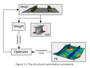
The existence of efficient optimization algorithms does guaranty that the problem of optimum design will be successfully addressed. The experience of the engineer is important parameter for the proper use of these algorithms. The design procedure is an iterative process where repetition is considered as the sequential test of candidate designs and evaluates whether they are superior or not compared to the past ones, while satisfying the constraints of the problem. The conventional procedure used by engineers is that of “trial and error”. Of course, with increased the complexity and magnitude of the problems the use of such empirical techniques does not lead to the optimal solution. So, it became necessary to automate the design of buildings by exploiting the developments in computer technology and the advances in optimization algorithms. Today, these tests can be performed automatically and with greater speed and accuracy. The optimum design procedure for structural systems is presented in Figure 1.1. ACE OCP is a general purpose and highly efficient software for performing sizing structural optimization and it is based on the most advanced numerical optimization algorithms (Lagaros, 2014).

1.2   Formulation of the Structural Optimization Problem

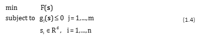
Structural optimization problems are characterized by various objective and constraint functions that are generally non-linear functions of the design variables. These functions are usually implicit, discontinuous and non-convex. The mathematical formulation of structural optimization problems with respect to the design variables, the objective and constraint functions depend on the type of the application. However, all optimization problems can be expressed in standard mathematical terms as a non-linear programming problem (NLP), which in general form can be stated as follows.

where, s is the vector of design variables, F(s) is the objective function to be minimized, g_j are the behavioral constraints, s^l and s^u are the lower and the upper bounds on the i^th design variable. Equality constraints are usually rarely imposed. Whenever they are used they are treated for simplicity as a set of two inequality constraints.

To address a problem of mixed optimal design many methods have been developed. Usually in the case of a mixed-discrete or a purely discrete problem the design variables are dealt as though they were continuous design variables; while at the end of the process, once the optimal values of all design variables have been determined, appropriate values derived from the discrete design space are assigned to the continuously defined design variables. For the case of a discrete optimal design problem in which the design space can be sorted according to all cross-sectional characteristics (cross section area, main and secondary moments of inertia, etc.) in a strictly monotonic sequence, this technique provides a better approximation of the optimal solution. But in practical problems this is not the case. The work of Bremicker et al. (1990) presents an overview of the main methods for the treatment of the mixed-discrete optimum design problems.

1.2.1    Design Variables

The parameters, that when their values are obtained the design if fully defined, are called design variables. If a design does not fulfill the design requirements of the problem then it is called infeasible, otherwise it is known as a feasible design. One feasible design is not necessarily the best but it can always be implemented. A very important first step for proper formulation of a problem is the correct selection of the design variables. In cases where the selection of the design variables is not correct then the formulation may be incorrect or in the worst case, the optimal design obtained from the optimization algorithm is not feasible. Although this way the “degrees of freedom” of the formulation of the optimization problem of the system is increased, there are cases that it is desirable to select more design variables that are necessary for the proper formulation of the problem. In such problems, it is possible to remove the additional design variables by designating to them specific values for the next steps of the optimization procedure. Another important issue that needs to be taken into account in the selection of design variables is their relative independence.

 

During the formulation of the mathematical optimization model the function to be optimize should be sufficiently dependent on all the design parameters. Let as consider the case that the objective function is the weight of the structure, where the minimum value is to be obtained and let assume that the magnitude of the weight is at the order of 1,000 Kg. If the weight of a structural member is in the order of 10^-3 Kg or less and let as consider that this member represents one of the design variables of the problem, then if the value is changed by 100% the influence on the value of the objective function is negligible. To avoid conditions, such as those mentioned above, it is necessary that linkage between the design variables is implemented. Therefore, some members of the structure can be represented by a common design parameter. Therefore, it is recommended to conduct a sensitivity analysis in order to estimate the sensitivity of the objective function over all the design parameters before the final choice of the optimization model. Through the sensitivity analysis it is possible to detect design parameters that have negligible influence on the objective function.

 

1.2.2    Objective Functions

Every optimization problem is described by a large number of feasible designs and some of them are better and some others are worst while only one is the best solution. To make this kind of distinction between good and better designs it is necessary to have a criterion for comparing and evaluating the designs. This criterion is defined by a function that takes a specific value for any given design. This function is called as objective function, which depends on the design variables. With no violation of the generality the formulation given in Eq. (1.1) refers to a minimization problem. A maximizing problem of the function F(s) can be transformed into a minimization problem of the objective function -F(s). An objective function that is to be minimized it is often called as the cost function.

 

The appropriate selection of the objective function is a very important step in the process of mathematical model to that of the proper selection of the design variables. Some examples of objective functions reported in the literature are: minimizing the cost, weight optimization problem, energy losses problem and maximizing the profit. In many cases the formulation of the optimization problem is defined with the simultaneous optimization of two or more objective functions that are conflicting against each other. As an example, of this type of optimization problem is the case where the objective is to find an optimum design with minimum weight and simultaneously to have minimum stress or displacement in some parts of the structural system. These types of problems are called optimization problems with multiple objective functions (multi-objective design or Pareto optimum design).

1.2.3    Constraint Functions

The design of a structural system is achieved when the design parameters take specific values. Design can be considered any arbitrarily defined structural system, such as a circular cross section with a negative radius, or a ring cross section with a negative wall thickness, as well as any non-constructible building system. All engineering or code provisions are introduced in the mathematical optimization model in the form of inequalities and equalities, which are called constraint functions. These constraint functions in order to have meaningful contribution on the mathematical formulation of the problem should be at least dependent on one design variable. The constraint functions that are usually imposed on structural problems are stress and strain constraints, whose values are not allowed to exceed certain limits. Sometimes the engineers impose additional constraint functions that may be useless, which they are either dependent on others or they remain forever in the safe area, this is due to the existence of uncertainties on the definition of the problem or due to inexperience. The use of additional constraint functions may result to calculations requiring additional computational effort without any benefit especially in the case of mathematical programming methods that they require to perform sensitivity analysis.

One inequality constraint function g_j(s)≤0 is considered as active at the point s^* in the case that the equality is satisfied, i.e. g_j(s^*)=0. Accordingly, the above constraint function is considered as inactive for the design s^* for the case that the inequality is strictly satisfied, i.e. g_j(s^*)<0. The inequality constraint function is considered that it is violated for the design s^* if a positive value that g_j(s^*)>0, corresponds to the value of the constraint function. Similarly, an equality constraint function h_j(s)=0 is considered that it is violated for the design s^* if the equality is not satisfied, i.e. h_j(s^*)=0. Therefore, an equality constraint function might be active or violated. From all the description provided related to the active or the inactive constraint functions it is clear that any feasible design is defined by active or inactive inequality constraint functions and active equality constraint functions.

At each step of the optimization process it is unlikely that all constraint functions are active. The engineers are not able to determine in advance which of these functions will become active and which of them will become inactive at each step. For this reason, when solving optimization problems, it is necessary to use different techniques to address more effectively the constraint functions, techniques that greatly improves the efficiency of the optimization procedure and reduce significantly the time required for the calculations. Especially when the problem is relatively large, i.e. the formulation of the problem is defined with many design variables and constraint functions, any possibility of reducing the calculations of the values required and the derivatives of constraint functions has significant impact on the efficiency of the performance of the optimization procedure. So, it is crucial to identify at each step of the optimization procedure the constraint functions that are located within the safe area, i.e. they are inactive, which they do not affect the process of finding of an improved design in order to continue the optimization process with only the active constraint functions.

An active constraint function suggests that its presence significantly affects the improvement of the current design. By definition, the equality constraint functions should be fulfilled at each step of the optimization procedure; therefore, they are considered always among the active constraint functions (Arora, 1989; Gill and Murray, 1981). An active inequality constraint function means that at this stage should be fulfilled as equality or even approximately. When a constraint function is inactive then it means that its presence is not important at that part of the optimization procedure, since the active constraint functions fulfill the needs of the design. This does not mean, though, that this constraint function is redundant as in another optimization step can be activated. Usually, in order to increase the effectiveness of the mathematical algorithms, only the active constraint functions are taken into account. On the other hand, other optimal design methods like the fully stressed design method are based on exploiting the presence of active constraint functions.

In order to identify the active constraint functions the values of the constraint functions should be normalized first (Vanderplaats, 1984) to have a single reference system regardless of the type of the constraint function. For example, it is likely that the value of a displacement constraint function to take values in the order of 0.1-2.0 cm, while the value of a stress displacement constraint function to take values is in the order of 25,000 kPa, so readily it is apparent that it is necessary to homogenize the sizes of the two constraint functions. The normalization of the value constraint functions takes place in accordance with the following relations:

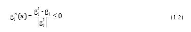
for a constraint function limited with a lower bound and:

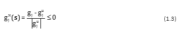
for a constraint function limited with an upper bound. Thus, if the normalized value of the constraint function is equal to +0.50 then it violates its permissible value by 50%, while if its normalized value is equal to -0.50 then this constraint is 50% below the allowable value. Usually among the active constraint functions are included those with normalized value greater than -0.1 to -0.01 (Arora, 1989). Furthermore, it is also allowed a small tolerance when the constraint functions violate the minimum allowable value (-0.005 to 0.001) since the process of simulation, analysis, design and construction involves many uncertainties.

 

1.2.4    Global and local minimum

A common problem for all mathematical optimization methods is that due to the deterministic nature of the operators used they may be directed to identifying a local minimum, in contrast to the methods that are based on probabilistic operators where random search procedures are implemented and they are more likely to locate the global minimum of the problem at hand. The definitions of the local and the global minimum in mathematical terms can be as follows:

Local minimum. A point s^* in the design space is considered as a local or a relative minimum if this design satisfies the constraint functions and the relationship F(s^*)≤F(s) is valid for every feasible design point in a small region around the point s^*. If only the inequality is valid, F(s^*)<F(s), then the point s^* is called as a strict or a unique or a strong local minimum.

Global minimum. A point s^* the design space is defined as the global or absolute minimum for the problem at hand if this design satisfies the constraint functions and the relation F(s^*)≤F(s) is valid for every feasible design point. If only the inequality is valid, F(s^*)<F(s), then the point s^* is called as a strict or a unique or a strong global minimum.

If there is no constraint functions then the same definitions can be used, but they are valid throughout the design space and they are not restricted only in the region of feasible designs. Generally, it is difficult to foretell in advance the existence of local or global minimum in every optimal design problem. However, if the objective function F(s) is continuous and the region of feasible designs is nonempty, closed and bounded, then there is a global minimum for the objective function F(s) (Arora, 1990). The region of feasible designs is defined as not empty when there are no conflicting constraint functions or when there are not redundant constraint functions. If the optimization algorithm cannot to identify any feasible point, then it can be said that the region of feasible designs is empty and therefore the problem should be reformulated by removing or defining some constraint functions to be more flexible. The region of feasible designs is defined as closed and fixed when the constraint functions are continuous and there are not “strict” inequality constraint functions (g(s)<0). The existence of minimum designs is not cancelled if these conditions are not satisfied, simply the minimum designs cannot be established mathematically, but these optimum designs can be obtained during the optimization process.

1.3   Classes of Structural Optimization

There are mainly three classes of structural optimization problems: sizing, shape and topology or layout. Initially structural optimization was focused on sizing optimization, such as optimizing cross sectional areas of truss and frame structures, or the thickness of plates and shells. The next step was to consider finding optimum boundaries of a structure, and therefore to optimize its shape. In the former case the structural domain is fixed, while in the latter case it is not fixed but it has a predefined topology. In both cases a non-optimal starting topology can lead to sub-optimal results. To overcome this deficiency structural topology optimization needs to be employed, which allows the designer to optimize the layout or the topology of a structure by detecting and removing the low-stressed material in the structure which is not used effectively.

1.3.1    Sizing Optimization

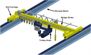
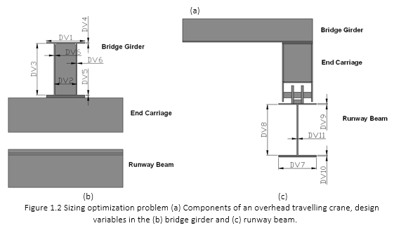
In sizing optimization problems, the aim is usually to minimize the weight of the structure under certain behavioral constraints on stresses and displacements. The design variables are most frequently chosen to be dimensions of the cross-sectional areas of the members of the structure. Due to engineering practice demands the members are divided into groups having the same design variables. This linking of elements results in a trade-off between the use of more material and the need of symmetry and uniformity of structures due to practical considerations. Furthermore, it has to be taken into account that due to fabrication limitations the design variables are not continuous but discrete since cross-sections belong to a certain set.

A discrete structural optimization problem can be formulated in the following form:

where R^d is a given set of discrete values representing the available structural member cross-sections and design variables s_i (i=1,…,n) can take values only from this set.

 

The sizing optimization methodology proceeds with the following steps: (i) At the outset of the optimization the geometry, the boundaries and the loads of the structure under investigation have to be defined. (ii) The design variables, which may or may not be independent to each other, are also properly selected. Furthermore, the constraints are also defined in this stage in order to formulate the optimization problem as in Eq. (1.4). (iii) A finite element analysis is then carried out and the displacements and stresses are evaluated. (iv) The design variables are being optimized. If the convergence criteria for the optimization algorithm are satisfied, then the optimum solution has been found and the process is terminated, else the optimizer updates the design variable values and the whole process is repeated from step (iii). A typical sizing optimization problem is presented in Figure 1.2.

1.3.2    Shape Optimization

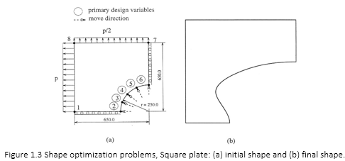
In structural shape optimization problems, the aim is to improve the performance of the structure by modifying its boundaries. This can be numerically achieved by minimizing an objective function subjected to certain constraints. All functions are related to the design variables, which are some of the coordinates of the key points in the boundary of the structure. The shape optimization approach adopted in the present software is based on a previous work by Hinton and Sienz for treating two-dimensional problems. More specifically the shape optimization methodology proceeds with the following steps: (i) At the outset of the optimization, the geometry of the structure under investigation has to be defined. The boundaries of the structure are modeled using cubic B-splines that, in turn, are defined by a set of key points. Some of the coordinates of these key points will be the design variables which may or may not be independent to each other. (ii) An automatic mesh generator is used to create a valid and complete finite element model. A finite element analysis is then carried out and the displacements and stresses are evaluated. (iii) If a gradient-based optimizer is used then the sensitivities of the constraints and the objective function to small changes of the design variables are computed either with the finite difference, or with the semi-analytical method. (iv) The optimization problem is solved; the design variables are being optimized and the new shape of the structure is defined. If the convergence criteria for the optimization algorithm are satisfied, then the optimum solution has been found and the process is terminated, else a new geometry is defined and the whole process is repeated from step (ii). A typical shape optimization problem is presented in Figure 1.3.

1.3.3    Topology Optimization

Structural topology optimization assists the designer to define the type of structure, which is best suited to satisfy the operating conditions for the problem in question. It can be seen as a procedure of optimizing the rational arrangement of the available material in the design space and eliminating the material that is not needed. Topology optimization is usually employed in order to achieve an acceptable initial layout of the structure, which is then refined with a shape optimization tool. The topology optimization procedure proceeds step-by-step with a gradual “removal” of small portions of low stressed material, which are being used inefficiently. This approach is treated in ACE OCP as a typical case of a structural reanalysis problem with small variations of the stiffness matrix between two subsequent optimization steps.

 

Many researchers have presented solutions for structural topology optimization problems. Topological or layout optimization can be undertaken by employing one of the following main approaches, which have evolved during the last few years: (i) Ground structure approach, (ii) homogenization method, (iii) bubble method and (iv) fully stressed design technique. The first three approaches have several things in common. They are optimization techniques with an objective function, design variables, constraints and they solve the optimization problem by using an algorithm based on sequential quadratic programming (approach (i)), or on an optimality criterion concept (approaches (ii) and (iii)). However, inherently linked with the solution of the optimization problem is the complexity of these approaches. The fully stressed design technique on the other hand, although not an optimization algorithm in the conventional sense, proceeds by removing inefficient material, and therefore optimizes the use of the remaining material in the structure, in an evolutionary process. A typical shape optimization problem is presented in Figure 1.4.

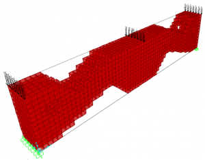Figure 1.4 Topology optimization for a single loading condition

1.4   Metaheuristic Optimization

Heuristic algorithms are based on trial-and-error, learning and adaptation procedures in order to solve problems. Metaheuristic algorithms achieve efficient performance for a wide range of combinatorial optimization problems. Computer algorithms based on the process of natural evolution have been found capable to produce very powerful and robust search mechanisms although the similarity between these algorithms and the natural evolution is based on crude imitation of biological reality. The resulting Evolutionary Algorithms (EA) are based on a population of individuals, each of which represents a search point in the space of potential solutions of a given problem. These algorithms adopt a selection process based on the fitness of the individuals and some recombination operators. The best-known EA in this class include evolutionary programming (EP), Genetic Algorithms (GA) and Evolution Strategies (ES). The first attempt to use evolutionary algorithms took place in the sixties by a team of biologists and was focused in building a computer program that would simulate the process of evolution in nature.

Both GA and ES imitate biological evolution in nature and have three characteristics that differ from other conventional optimization algorithms: (i) In place of the usual deterministic operators, they use randomized operators: mutation, selection and recombination. (ii) Instead of a single design point, they work simultaneously with a population of design points in the space of design variables. (iii) They can handle, with minor modifications continuous, discrete or mixed optimization problems. The second characteristic allows for natural implementation of GA and ES on a parallel computing environment.

In structural optimization problems, where the objective function and the constraints are highly non-linear functions of the design variables, the computational effort spent in gradient calculations required by the mathematical programming algorithms is usually large. In two recent studies by Papadrakakis et al. it was found that probabilistic search algorithms are computationally efficient even if greater number of analyses is needed to reach the optimum. These analyses are computationally less expensive than in the case of mathematical programming algorithms since they do not need gradient information. Furthermore, probabilistic methodologies were found, due to their random search, to be more robust in finding the global optimum, whereas mathematical programming algorithms may be trapped in local optima.

 

1.4.1    Genetic Algorithms

GA are probably the best-known evolutionary algorithms, receiving substantial attention in recent years. The GA model used in ACE OCP and in many other structural design applications refers to a model introduced and studied by Holland and co-workers. In general, the term genetic algorithm refers to any population-based model that uses various operators (selection-crossover-mutation) to evolve. In the basic genetic algorithm, each member of this population will be a binary or a real valued string, which is sometimes referred to as a genotype or, alternatively, as a chromosome. Different versions of GA have appeared in the literature in the last decade dealing with methods for handling the constraints or techniques to reduce the size of the population of design vectors. In this section the basic genetic algorithms together with some of the most frequently used versions of GA are considered.

The three main steps of the basic GA

Step 0 Initialization

The first step in the implementation of any genetic algorithm is to generate an initial population. In most cases the initial population is generated randomly. In ACE OCP in order to perform a comparison between various optimization techniques the initial population is fixed and is chosen in the neighborhood of the initial design used for the mathematical programming methods. After creating an initial population, each member of the population is evaluated by computing its fitness function.

Step 1 Selection

Selection operator is applied to the current population to create an intermediate one. In the first generation, the initial population is considered as the intermediate one, while in the next generations this population is created by the application of the selection operator.

Step 2 Generation

In order to create the next generation crossover and mutation operators are applied to the intermediate population to create the next population. Crossover is a reproduction operator, which forms a new chromosome by combining parts of each of the two parental chromosomes. Mutation is a reproduction operator that forms a new chromosome by making (usually small) alterations to the values of genes in a copy of a single parent chromosome. The process of going from the current population to the next population constitutes one generation in the evolution process of a genetic algorithm. If the termination criteria are satisfied the procedure stops otherwise returns to step 1.

Encoding

The first step before the activation of any operator is the step of encoding the design variables of the optimization problem into a string of binary digits (l’s and 0’s) called a chromosome. If there are n design variables in an optimization problem and each design variable is encoded as a L-digit binary sequence, then a chromosome is a string of n´L binary digits. In the case of discrete design variables each discrete value is assigned to a binary string, while in the case of continuous design variables the design space is divided into a number of intervals (a power of 2). The number of intervals L+1 depends on the tolerance given by the designer. If sÎ[s^l, s^u] is the decoded value of the binary string <b_Lb_L-1…b₀> then:

where DE(.) is the function that performs the decoding procedure. In order to code a real valued number into the binary form the reverse procedure is followed.

Selection

There are a number of ways to perform the selection. According to the Tournament Selection scheme each member of the intermediate population is selected to be the best member from a randomly selected group of members belonging to the current population. According to the Roulette Wheel selection scheme, the population is laid out in random order as in a pie graph, where each individual is assigned space on the pie graph in proportion to fitness. Next an outer roulette wheel is placed around the pie with N equally spaced pointers, where N is the size of the population. A single spin of the roulette wheel will now simultaneously pick all N members of the intermediate population.

Crossover

Crossover is a reproduction operator, which forms a new chromosome by combining parts of each of two ‘parent’ chromosomes. The simplest form is called single-point crossover, in which an arbitrary point in the chromosome is picked. According to this operator two ‘offspring’ chromosomes are generated, the first one is generated by copying all the information from the startup of the parent A to the crossover point and all the information from the crossover point to the end of parent B. The second ‘offspring’ chromosome is generated by the reverse procedure. Variations exist which use more than one crossover point, or combine information from parents in other ways.

Mutation

Mutation is a reproduction operator, which forms a new chromosome by making (usually small) alterations to the values of genes in a copy of a single parent chromosome.

1.4.2    Evolution Strategies

ES were proposed for parameter optimization problems in the seventies by Rechenberg and Schwefel. Some differences between GA and ES stem from the numerical representation of the design variables used by these two algorithms. The basic GA operates on fixed-sized bit strings which are mapped to the values of the design variables, ES work on real-valued vectors. Another difference can be found in the use of the genetic operators. Although, both GA and ES use the mutation and recombination (crossover) operators, the role of these genetic operators is different. In GA mutation only serves to recover lost alleles, while in ES mutation implements some kind of hill-climbing search procedure with self-adapting step sizes σ (or γ). In both algorithms recombination serves to enlarge the diversity of the population, and thus the covered search space. There is also a difference in treating constrained optimization problems where in the case of ES the death penalty method is always used, while in the case of GA only the augmented Lagrangian method can guarantee the convergence to a feasible solution. The ES, however, achieve a high rate of convergence than GA due to their self-adaptation search mechanism and are considered more efficient for solving real world problems.

Multi-membered ES

According to the multi-membered evolution strategies a population of μ parents will produce λ offsprings. Thus, the two steps are defined as follows:

Step 1 (recombination and mutation).

The population of μ parents at g^th generation produces λ offsprings. The genotype of any descendant differs only slightly from that of its parents.

Step 2 (selection).

There are two different types of the multi-membered ES:

(μ+λ)-ES: The best μ individuals are selected from a temporary population of (μ+λ) individuals to form the parents of the next generation.

(μ,λ)-ES:  The μ individuals produce λ offsprings (μ<λ) and the selection process defines a new population of μ individuals from the set of λ offsprings only.

In the second type, the existence of each individual is limited to one generation. This allows the (μ,λ)-ES selection to perform better on problems with an optimum moving over time, or on problems where the objective function is noisy.

In Step 1, for every offspring vector a temporary parent vector  is first built by means of recombination. For continuous problem, the following recombination cases can be used

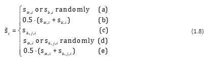
where  is the i^th component of the temporary parent vector , s_α,i and s_b,i are the i^th components of the vectors s_a and s_b which are two parent vectors randomly chosen from the population. In case (c),  means that the i^th component of  is chosen randomly from the i^th components of all μ parent vectors. From the temporary parent  an offspring can be created in the same way as in two-membered ES.

ES in structural optimization problems

The ES optimization procedure starts with a set of parent vectors and if any of these parent vectors gives an infeasible design then this parent vector is modified until it becomes feasible. Subsequently, the offsprings are generated and checked if they are in the feasible region. The computational efficiency of the multi-membered ES is affected by the number of parents and offsprings involved. It has been observed that values of μ and λ should be close the number of the design variables produce best results.

 

The ES algorithm for structural optimization applications can be stated as follows:

1. Selection step: selection of the parent vectors of the design variables.
2. Analysis step: solve K(s_i)u_i=f (i=1,2,…,μ), where K is the stiffness matrix of the structure and f is the loading vector.
3. Constraints check: all parent vectors become feasible.
4. Offspring generation: generate the offspring vectors of the design variables.
5. Analysis step: solve K(s_j)u_j=f (j=1,2,…,λ).
6. Constraints check: if satisfied continue, else change s­_j and go to step 4.
7. Selection step: selection of the next generation parents according to (μ+λ) or (μ,λ) selection schemes.
8. Convergence check: If satisfied stop, else go to step 3.

1.4.3    Methods for Handling the Constraints

Although genetic algorithms are initially developed to solve unconstrained optimization problems during the last decade several methods have been proposed for handling constrained optimization problems as well. The methods based on the use of penalty functions are employed in the majority of cases for treating constraint optimization problems with GA. In ACE OCP methods belonging to this category have been implemented and will be briefly described in the following paragraphs.

Method of static penalties

In this simple method, the objective function is modified as follows

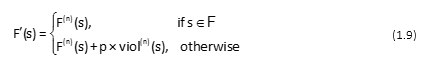
where p is the static penalty parameter, viol⁽ⁿ⁾ is the sum of the violated constraints

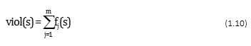
and F⁽ⁿ⁾ is the objective function to be minimized, both normalized in [0,1], while F is the feasible region of the design space.

 

The sum of the violated constraints is normalized before it is used for the calculation of the modified objective function. The main advantage of this method is its simplicity. However, there is no guidance on how to choose the single penalty parameter p. If it is chosen too small the search will converge to an infeasible solution otherwise if it is chosen too large a feasible solution may be located but it would be far from the global optimum. A large penalty parameter will force the search procedure to work away from the boundary, where is usually located the global optimum, that divides the feasible region from the infeasible one.

Method of dynamic penalties

The method of dynamic penalties was proposed by Joines and Houck and applied to mathematical test functions. As opposed to the previous method, the penalty parameter does not remain constant during the optimization process. Individuals are evaluated (at the generation g) by the following formula

 

with

where c, α and β are constants. A reasonable choice for these parameters was proposed as follows: c = 0.5 to 2.0, α = β =1 or 2. For high generation number, however, the (c×g)α component of the penalty term takes extremely large values which makes even the slightly violated designs not to be selected in subsequent generations. Thus, the system has little chances to escape from local optima. In most experiments reported by Michalewicz the best individual was found in early generations.

Augmented Lagrangian method

According to the Augmented Lagrangian method (AL-GA) the constrained problem is transformed to an unconstrained one, by introducing two sets of penalty coefficients γ [(γ₁,γ₂,…,γ_Μ+Ν)] and μ [(μ₁,μ₂,…,μ_Μ+Ν)]. The modified objective function, for the generation g, is defined as follows:

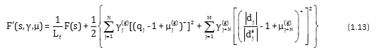
where L_f is a factor for normalizing the objective function; q_j is a non-dimensional ratio related to the stress constraints of the j^th element group; d_j is the displacement in the direction of the j^th examined degree of freedom, while  is the corresponding allowable displacement; N, M correspond to the number of stress and displacement constraint functions, respectively:

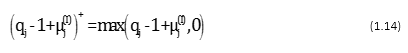
and

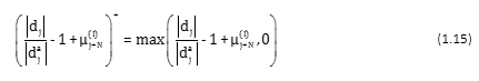
There is an outer step I and the penalty coefficients are updated at each step according to the expressions  and  where  and  is the average value of the j^th constraint function for the I^th outer step, while the initial values of γ’s and μ’s are set equal to 3 and zero, respectively. Coefficient β is taken equal to 10 as recommended by Belegundu and Arora.

 

1.5   References

Arora J.S., (1990) Computational Design Optimization: A review and future directions, Structural Safety, 7, 131-148.
Arslan M.A. Hajela P. Counterpropagation Neural Networks in decomposition based optimal design, Computers & Structures, 65(5), pp. 641-650, 1997.
Back T., Hoffmeister F. Schwefel H.-P., A survey of evolution strategies, in R.K. Belew and L. B. Booker (eds.), Proceedings of the 4th International Conference on Genetic Algorithms, Morgan Kaufmann, 2-9, (1991).
Baker J., Adaptive selection methods for genetic algorithms, in J. J. Grefenstette (ed.), Proc. International Conf. On Genetic Algorithms and their applications, Lawrence Erlbaum, (1985).
Barricelli N.A., Numerical testing of evolution theories, ACT A Biotheoretica, 16, 69-126, (1962).
Belegundu A.D., Arora J.S., A computational study of transformation methods for optimal design, AIAA Journal, 22(4), 535-542, (1984).
Bendsoe M.P., Kikuchi N., Generating optimal topologies in structural design using a homogenization method, Computer Methods in Applied Mechanics and Engineering, 71, 197-224, 1988.
Berke L., Hajela P., (1990) Applications of Artificial Neural Nets in Structural Mechanics, NASA 331-348 TM-102420.
Berke L., Patnaik S.N., Murthy P.L.N., Optimum Design of Aerospace Structural Components using Neural Networks, Computers & Structures, 48, pp. 1001-1010, 1993.
Bletzinger K.U., Kimmich S., Ramm E., (1991) Efficient modeling in shape optimal design, Computing Systems in Engineering, 2(5/6), 483-495.
Cai J. Thierauf G., Discrete structural optimization using evolution strategies, in B.H.V. Topping and A.I. Khan (eds.), Neural networks and combinatorial in civil and structural engineering, Edinburgh, Civil-Comp Limited, 95-10, (1993).
Embrechts M.J., Metaneural-Version 4.1, Rensselear Polytechnique Institute, 1994.
Eschenauer H.A., Schumacher A., Vietor T., Decision makings for initial designs made of advanced materials, in Bendsoe M.P. and Soares C.A.M. (eds.), NATO ARW Topology design of structures, Sesimbra, Portugal, Kluwer Academic Publishers, Dordrecht, Netherlands, 469-480, 1993.
Fleury C., (1993) Dual methods for convex separable problems, in Rozvany G.I.N. (ed), NATO/DFG ASI `Optimization of large structural systems’, Berchtesgaden, Germany, Kluwer Academic Publishers, Dordrecht, Netherlands, 509-530.
Fogel L.J., Owens A.J., and Walsh M.J., (1966) Artificial intelligence through simulated evolution, Wiley, New York.
Gallagher R.H., Zienkiewicz O.C., Optimum Structural Design: Theory and Applications, John Wiley & Sons, New York, 1973.
Gill P.E, Murray W., Wright M.H., (1981) Practical Optimization, Academic Press.
Goldberg D., A note on boltzmann tournament selection for Genetic Algorithms and population-oriented Simulated Annealing, TCGA 90003, Engineering Mechanics, Alabama University, (1990).
Goldberg D.E., (1989) Genetic algorithms in search, optimization and machine learning, Addison-Wesley Publishing Co., Inc., Reading, Massachusetts.
Goldberg D.E., Sizing populations for serial and parallel genetic algorithms, TCGA Report No 88004, University of Alabama, (1988).
Gunaratnam D.J. Gero J.S. Effect of representation on the performance of Neural Networks in structural engineering applications, Microcomputers in Civil Engineering, Vol. 9, pp. 97-108, 1994.
Haug E.J. Arora J.S., Optimal mechanical design techniques based on optimal control methods, ASME paper No 64-DTT-10, Proceedings of the 1st ASME design technology transfer conference, 65-74, New York, October, 1974.
Hinton E., Hassani B., Some experiences in structural topology optimization, in B.H.V. Topping (ed.) Developments in Computational Techniques for Structural Engineering, CIVIL-COMP Press, Edinburgh, 323-331, 1995.
Hinton E., Sienz J., Fully stressed topological design of structures using an evolutionary procedure, Journal of Engineering Computations, 12, 229-244, 1993.
Hoffmeister F., Back T., (1991) Genetic Algorithms and Evolution Strategies-Similarities and Differences, in Schwefel, H.P. and Manner, R. (eds.), Parallel Problems Solving from Nature, Springel-Verlag, Berlin, Germany, 455-469.
Holland, John Henry 1975. Adaptation in natural and artificial systems: an introductory analysis with applications to biology, control, and artificial intelligence. University of Michigan Press.
Hooke R. Jeeves T.A., ‘Direct Search Solution of Numerical and Statistical Problems’, J. ACM, Vol. 8, (1961).
Joines J. Houck C., On the use of non-stationary penalty functions to solve non- linear constrained optimization problems with GA, in Z. Michalewicz, J. D. Schaffer, H.-P. Schwefel, D. B. Fogel, and H. Kitano (eds.), Proceedings of the First IEEE International Conference on Evolutionary Computation, 579-584. IEEE Press, (1994).
Kennedy, J., & R. Eberhart 1995. Particle swarm optimization. In IEEE International Conference on Neural Networks, volume 4, pages 1942-1948.
Kirkpatrick, S., C. D. Gelatt, & M. P. Vecchi 1983. Optimization by Simulated Annealing. Science, 220(4598):671-680. PMID: 17813860.
Krishnakumar K., Micro genetic algorithms for stationary and non-stationary function optimization, in SPIE Proceedings Intelligent control and adaptive systems, 1196, (1989).
Lasdon L.S., Warren A.D., Jain A., Ratner R., (1978) Design and testing of a generalized reduced gradient code for nonlinear programming, ACM Trans. Math. Softw., 4 (1), 34-50.
Le Riche R. G., Knopf-Lenoir C. Haftka R. T., A segregated genetic algorithm for constrained structural optimization, in L. J. Eshelman (ed.), Proceedings of the 6th International Conference on Genetic Algorithms, 558-565, (1995).
Michalewicz Z., Genetic algorithms, numerical optimization and constraints, in L. J. Eshelman (ed.), Proceedings of the 6th International Conference on Genetic Algorithms, 151-158, Morgan Kaufmann, (1995).
Moses F., Mathematical programming methods for structural optimization, ASME Structural Optimization Symposium AMD Vol. 7, 35-48, 1974.
Myung H., Kim J.-H. Fogel D., ‘Preliminary investigation into a two-stage method of evolutionary optimization on constrained problems’, in J. R. McDonnell, R. G. Reynolds and D. B. Fogel (eds.), Proceedings of the 4th Annual Conference on Evolutionary Programming, 449-463, MIT Press, (1995).
Olhoff N., Rasmussen J., Lund E., (1992) Method of exact numerical differentiation for error estimation in finite element based semi-analytical shape sensitivity analyses, Special Report No. 10, Institute of mechanical Engineering, Aalborg University, Aalborg, DK.
Papadrakakis M., Lagaros N. D., Thierauf G. Cai J., Advanced Solution Methods in Structural Optimization Based on Evolution Strategies, J. Engng. Comput., 15(1), 12-34, (1998).
Papadrakakis M., Lagaros N.D. Tsompanakis Y., Optimization of large-scale 3D trusses using evolution strategies and neural networks, Special Issue of the International Journal of Space structures, Vol. 14(3), pp. 211-223, 1999.
Papadrakakis M., Lagaros N.D., Tsompanakis Y., Structural optimization using evolution strategies and neural networks, Comp. Meth. Appl. Mechanics & Engrg, Vol. 156, pp. 309-333, 1998.
Papadrakakis M., Tsompanakis Y., Lagaros N.D., Structural shape optimization using Evolution Strategies, Engineering Optimization Journal, Vol. 31, pp 515-540, 1999.
Pedersen P., Topology optimization of three dimensional trusses, in Bendsoe M.P., and Soares C.A.M. (eds.), NATO ARW `Topology design of structures’, Sesimbra, Portugal, Kluwer Academic Publishers, Dordrecht, Netherlands, 19-31, 1993.
Pope G.G., Schmit L.A. (eds.) Structural Design Applications of Mathematical Programming Techniques, AGARDOgraph 149, Technical Editing and Reproduction Ltd., London, February, 1971.
Ramm E., Bletzinger K.-U., Reitinger R., Maute K., (1994) The challenge of structural optimization, in Topping B.H.V. and Papadrakakis M. (eds) Advances in Structural Optimization, CIVIL-COMP Press, Edinburgh, 27-52.
Rechenberg I., (1973) Evolution strategy: optimization of technical systems according to the principles of biological evolution, Frommann-Holzboog, Stuttgart.
Rozvany G.I.N., Zhou M., Layout and generalized shape optimization by iterative COC methods, in Rozvany G.I.N. (ed.), NATO/DFG ASI `Optimization of large structural systems’, Berchtesgaden, Germany, Kluwer Academic Publishers, Dordrecht, Netherlands, 103-120, 1993.
Rummelhart D.E., McClelland J.L., Parallel Distributed Processing, Volume 1: Foundations, The MIT Press, Cambridge, 1986.
Schittkowski K., Zillober C., Zotemantel R., (1994) Numerical comparison of non-linear algorithms for structural optimization, Structural Optimization, 7, 1-19.
Schwefel H.-P. Rudolph G., Contemporary Evolution Strategies. in F. Morgan, A. Moreno, J. J. Merelo and P. Chacion (eds.). Advances in Artificial Life, Proc. Third European Conf. on Artificial Life Granada, Spain, June 4-6, Springer, Berlin, 893-907, (1995).
Schwefel H.P., (1981) Numerical optimization for computer models, Wiley & Sons, Chichester, UK.
Sheu C.Y. Prager W., Recent development in optimal structural design, Applied Mechanical Reviews, 21(10), 985-992, 1968.
Shieh R.C., Massively parallel structural design using stochastic optimization and mixed neural net/finite element analysis methods, Computing Systems in Engineering, Vol. 5, No. 4-6, pp. 455-467, 1994.
Spunt L., Optimum Structural Design, Prentice-Hall, Englewood Cliffs, New Jersey, 41-42, 1971.
Stephens, J.E., VanLuchene, D., Integrated assessment of seismic damage in structures, Microcomputers in Civil Engineering, Vol. 9(2), pp. 119-128, 1994.
Suzuki K., Kikuchi N., Layout optimization using the homogenization method, in Rozvany G.I.N. (ed.), NATO/DFG ASI `Optimization of large structural systems’, Berchtesgaden, Germany, Kluwer Academic Publishers, Dordrecht, Netherlands, 157-175, 1993.
Svanberg K. (1987). The method of moving asymptotes, a new method for structural optimization, Int. J. Num. Meth. Eng., 23, 359-373.
Taylor C.A., EQSIM, A program for generating spectrum compatible earthquake ground acceleration time histories, Reference Manual, Bristol Earthquake Engineering Data Acquisition and Processing System, December 1989.
Thanedar P.B., Arora J.S., Tseng C.H., Lim O.K., Park G.J., (1986) Performance of some SQP methods on structural optimization problems, Inter. Journal of Num. Meth. Engng, 23, 2187-2203.
Thierauf G., Cai J., (1995) A two level parallel evolution strategy for solving mixed-discrete structural optimization problems. The 21th ASME Design Automation Conference, Boston MA, September 17-221.
Thierauf G., Cai J., (1996) Structural optimization based on Evolution Strategy, in Papadrakakis M. and Bugeda G. (eds), Advanced computational methods in structural mechanics, CIMNE, Barcelona, 266-280.
Van Keulen F. Hinton E., Topology design of plate and shell structures using the hard kill method, in B.H.V. Topping (ed.) Advances in optimization for Structural Engineering, CIVIL-COMP Press, Edinburgh, 177-188, 1996.
Vanderplaats G.N., Numerical optimization techniques for engineering design: with applications, McGraw-Hill, New York, 1984.
Xie Y.M., Steven G.P., A simple evolutionary procedure for structural optimization, Computers & Structures, Vol. 49, 885-896, 1993.
Xie Y.M., Steven G.P., Optimal design of multiple load case structures using an evolutionary procedure, Journal of Engineering Computations, Vol. 11, 295-302, 1994.

1.6   Acronyms and Abbreviations

AL-GA: Augmented Lagrangian Genetic Algorithms
EA: Evolutionary Algorithms
EP: Evolutionary Programming
ES: Evolution Strategies
FSD: Fully Stressed Design
GA: Genetic Algorithms
M-ES: Multi-membered Evolution Strategy
NLP: Non-linear Programming Problem

Please read the full User’s Guide for more information